How To Create an Excel Drop Down List (2 Simple Ways) (2024)

I often use an Excel drop down list In my line of work to improve the efficiency of my data entry tasks by limiting my choices. This saves me a lot of time and prevents errors. I commonly use an Excel drop-down list for managing inventory, categorizing expenses, and selecting statuses of various tasks.

You can add a dropdown list in Excel using the Data validation menu by selecting a list as the allowed data. In this article, I’ll explain how to add an Excel drop-down list, add error messages, and move drop-down lists between other workbooks.

How To Make an Excel Drop Down List From a Range of Cells

If your drop-down list contains multiple options, creating a list in the spreadsheet and referencing it when making the drop-down menu is better. This can have a lot of benefits. You can reference a larger area and add options to the drop-down menu later.

This also adds the benefit of making your drop-down menus dynamic, meaning you can change the options anytime.

Here is how to create dynamic drop-down options in Excel:

1. Open the Microsoft Excel spreadsheet where you want to add the dynamic drop-down list.
2. Select the range of cells where you will add an Excel drop down list.

3. Click on the “Data tab”in the top ribbon, then on the “Data Validation”button in “Data Tools.”
4. Click “Data Validation”from the drop-down menu to open a new window.

5. Click the “Allow”option in the data validation dialog box and choose “List.”

6. For the “Source,” we will be adding the cell range.
   • To do this, click the “Up”arrow towards the right side of the textbox.
   • This will open another window.

7. Now, you can select the cell range with your cursor.
   • Click and drag your cursor to select the cell range for the drop-down.
8. With the cells selected, click the “Down”arrow towards the right side of the textbox.
   • This will add the cell range to the “Source.”
9. Click the “OK”button to save the changes.

This will create a data validationlist in Excel that you can change anytime.

How To Create an Excel Drop Down List With Yes/No Options

When creating an Excel drop down list, usually, it’s more convenient to choose a cell range containing the data for the drop-down list.

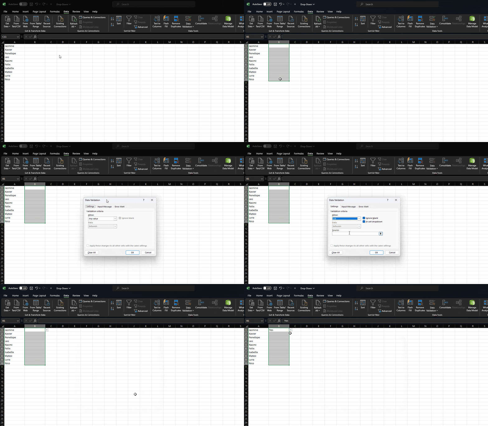
However, I recommend manually entering the data for the Excel yes/no drop-down lists with only a few inputs. Here is how to add an Excel drop-down list with only a few inputs:

1. Open the Excel spreadsheet where you want to create the in-cell dropdown list.
2. Select the cells where you want to insert the drop-down in Excel.
3. With the cells selected, click on “Data”in the top ribbon
4. Click on the “Data Validation”button in “Data Tools.”
   • This will open a small drop-down menu.
5. Select the “Data Validation”button to open a small window in the middle of the screen.
6. Here, you can select the “Validation criteria.”
   • Select the “Allow” option and click the “List”option.
   • This will change the selection options below.
7. Click on the “Source” text box below.
   • Here, I can write a list of drop-down options.
8. Enter the list of options separated by commas.
   • For example, I want the drop-down options to be “Yes”and “No.”
   • I will write them as “Yes,No.”
9. With the options added, click the “OK”button to save the changes.

A small arrow icon with the drop-down menu will now show towards the selected cell’s right side.

Note: This doesn’t have to be yes or no, but any defined names as list items.

Related Reading: How to Make Multiple Selections in Drop-down Lists in Google Sheets

Video Guide: Adding Drop Down Lists in Excel

How To Show Error for Invalid Data in Drop-Down Selection

Although drop-down menus allow users to choose the value they wish to add to the cells, you can still insert your values by simply clicking on the cell and typing.

To ensure unwanted values aren’t added, I can show an error alert if invalid data is added. Here is how to do this:

1. Open the Excel workbook and select the cells to add the error alert.

2. With the cells selected, click on “Data”in the top ribbon and choose the “Data Validation” option in the “Data Tools”section.
3. If you haven’t specified the drop-down list, specify the drop-down parameters in the “Settings” tab.

4. Once you do that, click the “Error Alert”tab.

5. Check the “Show error alert after invalid data is entered”option.

6. Below, you can choose the “Style”from “Stop, Warning, and Information.”
7. After choosing the type of pop-up, select the “Title” and the content of the “Error message.”
8. Once you add the data, click the “OK”button to save the changes.

Related Reading:Excel and Google Sheets Drop-down Lists

How To Remove an Excel Drop Down List

Now that we know how to add an Excel drop down list, let’s take a look at how to remove an Excel pick from the drop-down list:

1. Open the Excel workbook and select the cells to remove the drop-down.

2. With the cells selected, click on “Data”in the ribbon.
3. Click on the “Data Validation” option in the “Data Tools” section here.

4. In the “Data Validation”window, go to the “Settings”tab and click the “Clear All” button.
5. Click the “OK” button to save the changes.

Related Reading: How to Make a Dependent Drop-Down List in Google Sheets

How To Copy an Excel Drop Down List From Another Workbook

Often, you might want to copy a drop-down from your main spreadsheet to another workbook.

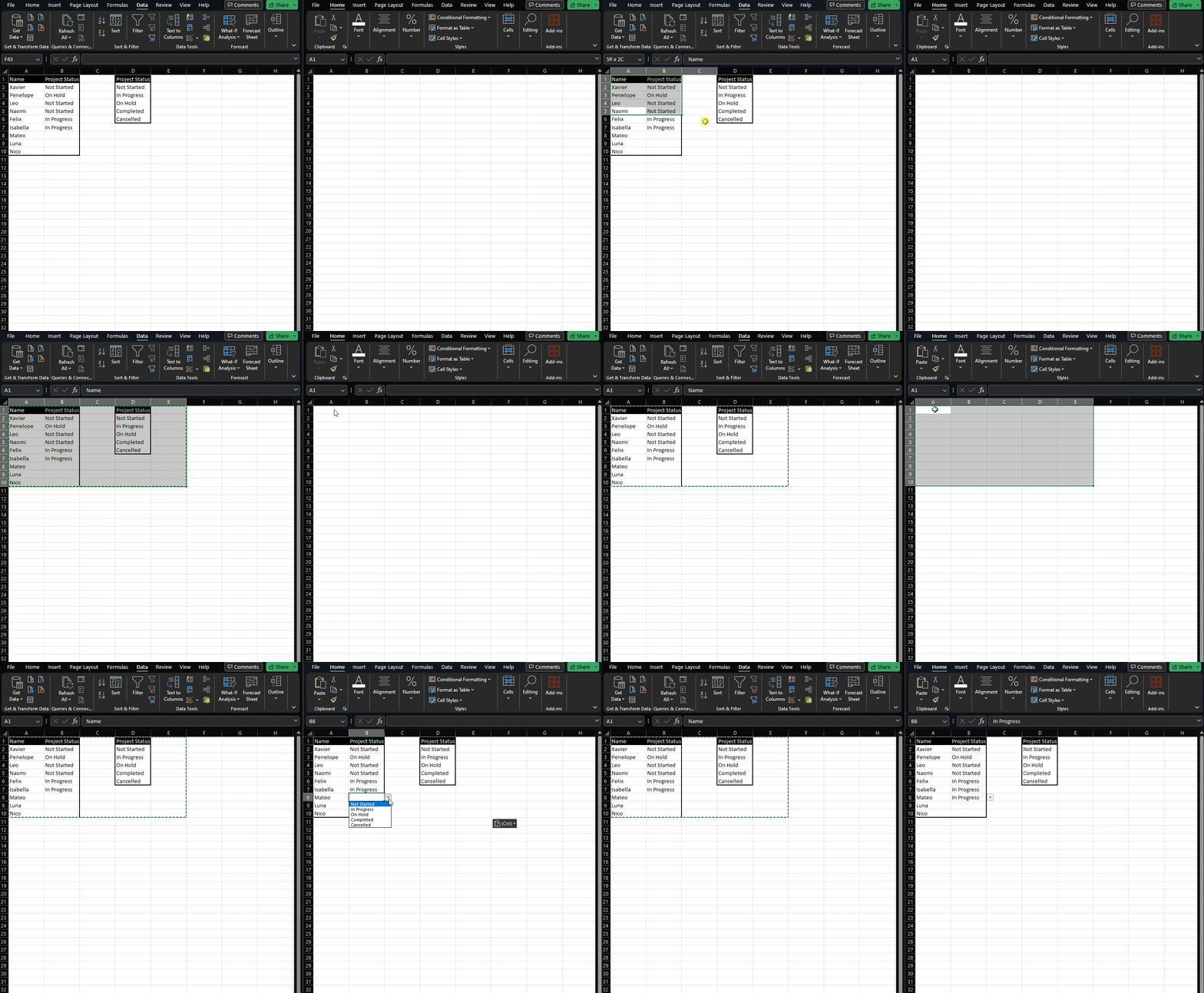
Thankfully, it’s straightforward to do this. Here is how to copy a drop-down list from one Excel spreadsheet to another:

1. Open the primary Excel workbook where you want to reproduce the Excel drop down list.
2. Here, select the cells containing the drop-down list.
3. With the cells selected, right-click on the cells and choose the “Copy”option.
   • You can also use the keyboard shortcut Ctrl + C (or Cmd + C on MacOS).
4. Now, head to the spreadsheet where you wish to paste the cells.
5. Here, click on the cell where you want to paste the cells.
   • The selected cell will be the top left cell of the table.
6. Now, right-click on the cell and choose the “Paste” option.
   • You can also use the keyboard shortcut Ctrl + Vto do this.

This will also work between worksheets in the same workbook.

Related Reading:Excel Tips and Tricks 2024: Optimize Your Workflow

Conclusion

An Excel drop down list is convenient because it improves data management efficiency. Whether you are categorizing expenses or selecting the status of a project, drop-down lists can help improve your workflow and reduce errors significantly, especially once you add error messages for invalid data.

Do you find Excel drop-down lists useful? What is the most creative way you’ve used an Excel drop-down list? Let us know in the comments below. Or, if you have any feedback for my tutorial, feel free to tell us in the comments.

Related:

• Master the Excel Break Links Feature in 5-Minutes
• How To Insert Multiple Rows in Excel
• Remove Blank Rows in Excel in a Few Easy Clicks